In the world of finance, risk is an inherent part of every investment decision. However, understanding and managing this risk is not always straightforward. This guide aims to demystify financial risk for self-directed investors by delving into the statistical foundations that financial risk is based on. We will explore the key role that probability distributions, such as the normal distribution, play in analyzing and comparing investment returns. By the end of this guide, you will be able to compare two different investment returns using a normal distribution. Let’s go!

Probability Concepts: Probability, Variance, and Standard Deviation

Probability is the chance of an event occurring and is represented by a value of 0 – 1; it is the likelihood of something happening. A probability of 1 means that the likelihood of an event occurring is 100%. This discussion is based on random variables; variables whose set of possible outcomes and their probabilities are known, but the actual outcome is not. Probability has 3 important features: 1) Exhaustive: Probability measuring from 0-1 means that it covers the entire range of outcomes, 2) Mutually Exclusive: only one event can occur at a time, 3) combining exhaustive and mutually exclusive events covers all possibilities (100%). For instance, flipping a coin is an intuitive way of understanding these features: 1) A coin has 2 sides so the probability of landing on either side covers the full range of possible outcomes, 2) Flipping a coin will only lead to either heads or tails but not both, 3) the probability of landing heads is 50% and the same for tails, therefore, the probability of both events together is 100%. This overly simplistic understanding of probability allows us to move on to probability distributions.

 Variance in statistics is a measure of how much the values in a data set differ from the average (mean). It is calculated by taking the average of the squared differences between each value and the mean (take each observation subtract it from the average, square it, sum all these observations up, and then divide by the number of observations). Variance expresses how spread out the data is and how far away or close to the mean. The higher the variance, the more dispersed the data are. The lower the variance, the more clustered the data are around the mean. Variance can be generally expressed mathematically as:

where:

• σ²: variance is expressed in squared units
• x_i​: represents each value in the data set,
• μ: is the mean of all values in the data set, and
• N: is the number of values in the data set,
• ∑: is a summation function (add up all the squared differences).

As you can see from the equation, variance is expressed in squared units, this means the answer reflects squared units. This is because variance represents how values differ from the mean in both directions. However, this is problematic when trying to use the data and the solution lies in standard deviation. Standard deviation is simply the square root of variance:

If variance represents the total variability around the mean, then standard deviation represents variability in only one direction from the mean. Thus, the standard deviation is usually expressed as ±. Now that we have a firm grasp of an event’s probability and how the event might deviate from the average, we can put it all together visually with a probability distribution.

The Normal Distribution

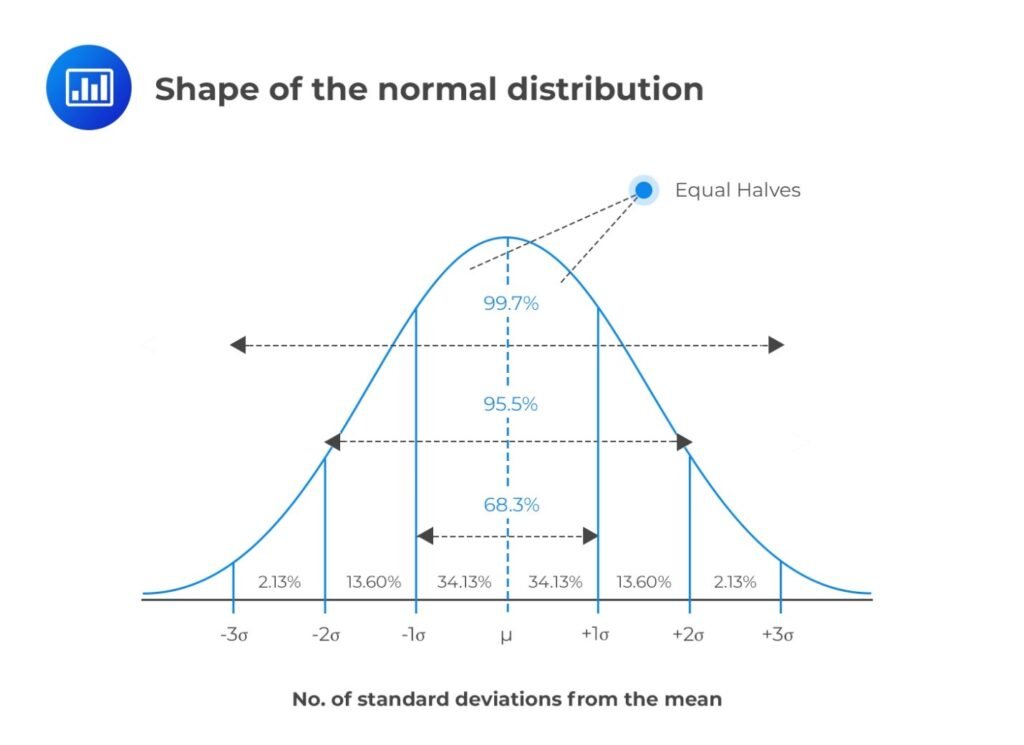
Source: Key Properties of the Normal distribution | CFA Level 1 – AnalystPrep

A probability distribution shows the likelihood of possible outcomes for a random variable—the probability of rolling a 4. A normal distribution is a probability distribution of a bell curve showing the likelihood of possible outcomes for a random variable symmetrically centered on the mean. The graph shown above from AnalystPrep is a good visual of the normal distribution, where the mean and its standard deviation are on the x-axis, and the y-axis represents the probability density function (the taller the curve the greater the likelihood). There are a couple defining characteristics of the normal distribution: It is completely described by two parameters mean, and variance (standard deviation), and it is symmetrical (skewness of 0). Based on our discussion of standard deviation, and by looking at the graph above, you can see that probabilities follow an empirical rule: approximately 68% of all observations fall in the interval μ ± 1σ (mean ± 1 standard deviation), 95% of observations fall within μ ± 2σ, and 99% of observations fall within μ ± 3σ. This rule combines probability with standard deviation and is visually expressed with the bell curve. Notice how the graph is tallest around the mean and shortest at the tails; a higher probability is associated with a lower standard deviation. In essence, the normal distribution visually expresses what is the most likely outcome of an event, and the likelihood it will deviate from that outcome.

Central Limit Theorem: Bridging The Gap Between Statistics And Returns

Critical data points for investors are stock returns, and the Central Limit Theorem (CLT) allows investors to apply the normal distribution to stock returns. CLT states that the sum of a large number of independent and identically distributed random variables, regardless of their distribution, will approximate a Normal Distribution—rolling dice 100 times would approximate a similar mean/distribution as rolling dice 1 million times. Thus, by assuming that stock returns are independent from day-today, that each daily return has the same probability of moving up or down, and that there are plenty of daily returns to satisfy a large number (30 is generally considered to be large), then we can input daily stock returns into a normal distribution. Let’s see how we can utilize the normal distribution to compare investments.

Example: Stocks vs Bonds

Stocks and bonds are key components in most portfolios. This is because stocks and bonds are negatively correlated, historically speaking. When stocks outperform, bonds underperform, and vice versa. They also have different characteristics: stocks typically offer higher returns but higher standard deviations, and bonds typically offer lower returns, but have a lower standard deviation. let’s look at how stocks and bonds performed in 2023: the S&P 500 Index as Stock A and the Bloomberg Barclays US Aggregate Bond Index as Bond B.

For the S&P 500 Index in 2023: Based on daily return data from Yahoo Finance, the average daily return was approximately 0.104%. The standard deviation of daily returns was approximately 1.52%. Using the properties of the normal distribution, we can calculate the probability of observing different ranges of daily returns for the S&P 500 Index:

• There is a 68% probability that the S&P 500 Index will have a daily return between -1.416% and 1.624% (one standard deviation from the mean).
• There is a 95% probability that the S&P 500 Index will have a daily return between -3.04% and 3.248% (two standard deviations from the mean).
• There is a 99.7% probability that the S&P 500 Index will have a daily return between -4.664% and 4.872% (three standard deviations from the mean).

Similarly, the Bloomberg Barclays US Aggregate Bond Index in 2023: The average daily return was approximately 0.021%. The standard deviation of daily returns was approximately 0.365%. We can perform the same calculations:

• There is a 68% probability that the Bloomberg Barclays US Aggregate Bond Index will have a daily return between -0.344% and 0.386% (one standard deviation from the mean).
• There is a 95% probability that the Bloomberg Barclays US Aggregate Bond Index will have a daily return between -0.709% and 0.751% (two standard deviations from the mean).
• There is a 99.7% probability that the Bloomberg Barclays US Aggregate Bond Index will have a daily return between -1.074% and 1.116% (three standard deviations from the mean).

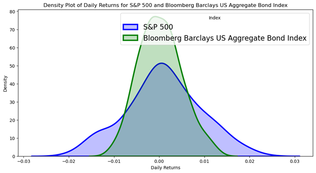
In graphical form:

Visually, the graph reveals obvious differences. The S&P500 graph is shorter, wider, and slightly more rightward shifted; a probability that reflects a higher return, lower chance of returning the mean, and wider dispersion (high risk—high reward). Whereas the bond index is taller, narrower, and less rightward shifted; a probability of a slightly lower return, a higher likelihood of returning the mean, and less dispersion (lower risk—lower return). This example highlights the universal concept in investing: stocks are riskier but offer higher returns, and bonds are safer but offer lower returns.  

Conclusion

In this article, we have learned how to use the normal distribution to analyze the risk and return of different investment options. We have seen that the normal distribution can be represented by a bell-shaped curve with a mean and a standard deviation that indicate the average and the variability of the data. We have also seen how to compare the graphs of two different normal distributions to see which one has higher or lower expected return, risk, and dispersion. Finally, we have applied these concepts to a practical example of comparing a stock index and a bond index using their historical returns and standard deviations. We have found that the stock index has higher return and risk, while the bond index has lower return and risk, consistent with the general trade-off between risk and reward in investing. By understanding the normal distribution and its properties, we can make better informed decisions about our portfolio allocation and diversification.